Disney BRDF
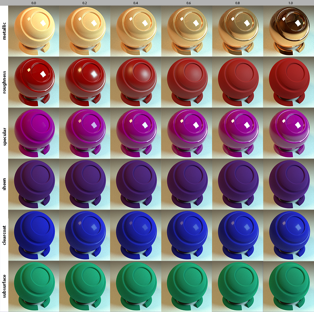
I wanted to be able to model a wide range of different surfaces. Therefore, the Disney's Principled BSDF was a logical choice, as it is a flexible surface appearance model. The model is not fully physically correct, but it was designed to allow a wide range of possible surfaces with as few parameters as possible. Some of these parameters can be seen in the image below, which is rendered using Nori:
Variables
To make sure all variables that are mentioned in the next paragraphs are clear.
Linear interpolation: \(lerp(t, a, b) = (1-t)a + tb\)
Diffuse Term
In the original Disney's BRDF paper the authors use the Schlick Fresnel approximation for the diffuse term and define the base diffuse model as: \[f_d=\frac{baseColor}{\pi}(1+(F_{D90}-1)(1-cos(\theta_i)^5)(1+(F_{D90}-1)(1-cos(\theta_o)^5)\] where \(F_{D90}=0.5+2 * roughness * cos^2(\theta_h)\).
Specular and Clearcoat Term
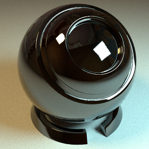
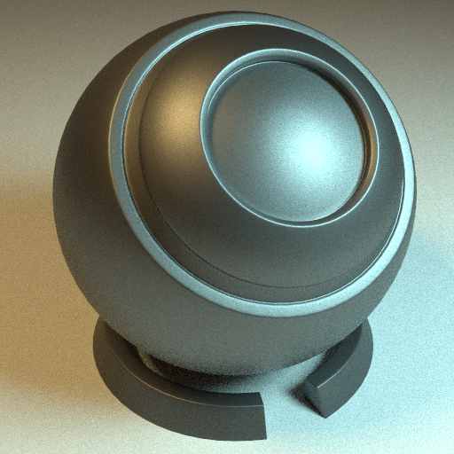
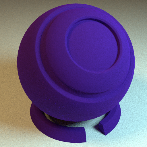
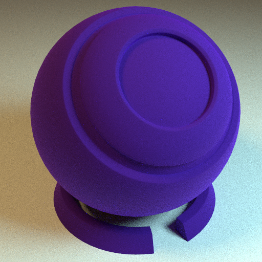
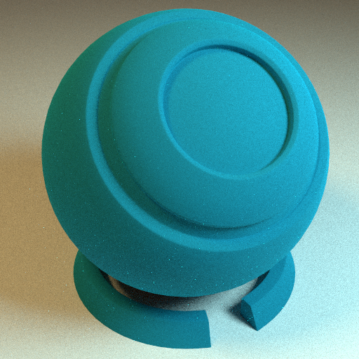
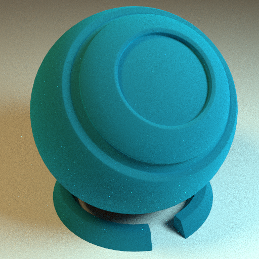
The Disney's BRDF uses the Microfacet model for the specular lobes with the Generalized-Trowbridge-Reitz (GTR) distribution as the normal distribution D For the specular lobe a value of \(\gamma = 2\) is used. \[f_s(\theta_i, \theta_o) = \frac{D_{GTR}(\theta_h) F(\theta_i) G(\theta_i, \theta_o)}{4cos(\theta_i)cos(\theta_o)}\] \[D_{GTR} = \frac{c}{(\alpha^2cos^2(\theta_h) + sin^2(\theta_h))^\gamma}\] \[\alpha = roughness^2\] The specular term controls the fresnel part of the model: \[F(\theta) = lerp((1-cos(\theta_D)^5), specularColor, 1)\] \[specularColor = lerp(metallic, 0.08 * specularTerm * mixTint, baseColor)\] \[mixTint = lerp(specularTint, 1, color\_tint)\] \[color\_tint = \frac{basecolor}{luminance}\] See below for a comparison of the roughness values 0.0 and 0.5 on metal surfaces and non metal surfaces:


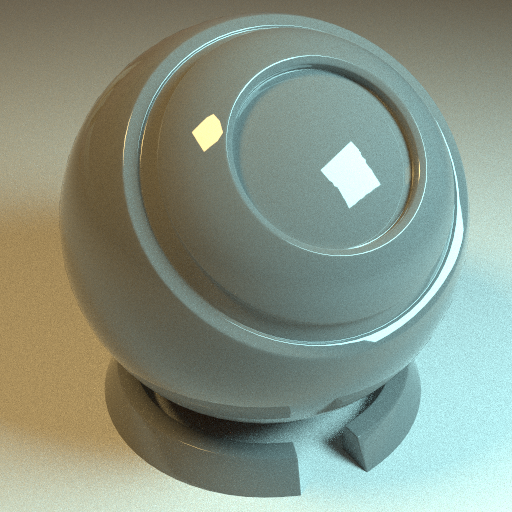


For the clearcoat lobe a second version of the GTR distribution is used with \(\gamma=1\). The IOR of the clearcoat is fixed to be 1.5 (value of polyurethane) and the strength of the clearcoat is defined by the clearcoat variable scaled to \([0..0.25]\). The roughness term for the clearcoat is defined as \(\alpha = lerp(clearcoatGloss, 0.2, 0.001)\). See below for a comparison of the clearcoat of Nori with Mitsuba. There is a small difference in brightness of the specularity of the clearcoat, which is caused by a slight differences in the implementation:
Sheen Term
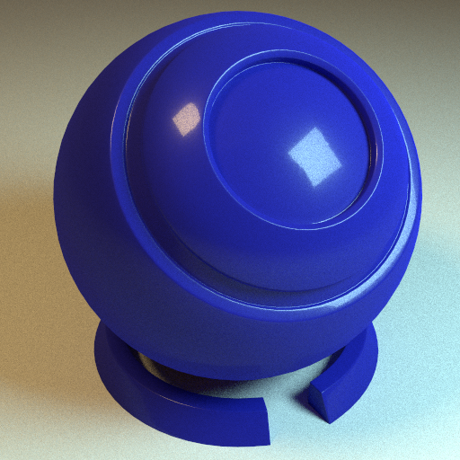
Sheen can typically be observed in cloth materials. The Disney's BRDF uses here the following term: \[f_{sheen} = F(\theta_h) * sheen * lerp(sheenTint, 1, baseColor)\] See below for a comparison of a sheen surface in Nori and Mitsuba.

Subsurface Term
Disney's BRDF blends between the diffuse term and a Hanrahan-Krueger inspired model and is an approximation to a physical correct subsurface scattering model with short free mean paths: \[diffuse_subsurface = lerp(subsurfaceTerm, diffuse, ss)\] \[ss = 1.25 *(Fss * (\frac{1}{cos(\theta_i)+cos(\theta_o)}-0.5)+0.5)\] \[Fss = lerp((1-cos(\theta_i)^5), 1, Fss90 ) * lerp((1-cos(\theta_o)^5), 1, Fss90 )\] \[Fss90 = cos(\theta_D)^2 * roughness\]
Importance Sample
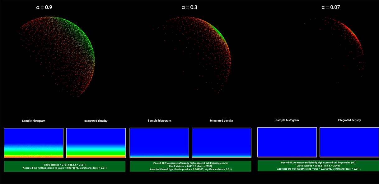
When sampling the BRDF the sampler decides to sample the diffuse or the specular lobe using the ratio \(\frac{1-metallic}{2}\). Diffuse samples are sampled from a cosine weighted hemisphere. Specular samples are again devided into GTR2 (specular) with \(\gamma=2\) and GTR (clearcoat) with \(\gamma=1\) using the ratio \(\frac{1}{1+clearcoat}\). To validate the sampling of GTR and GTR2, I used the warptest framework:
GTR: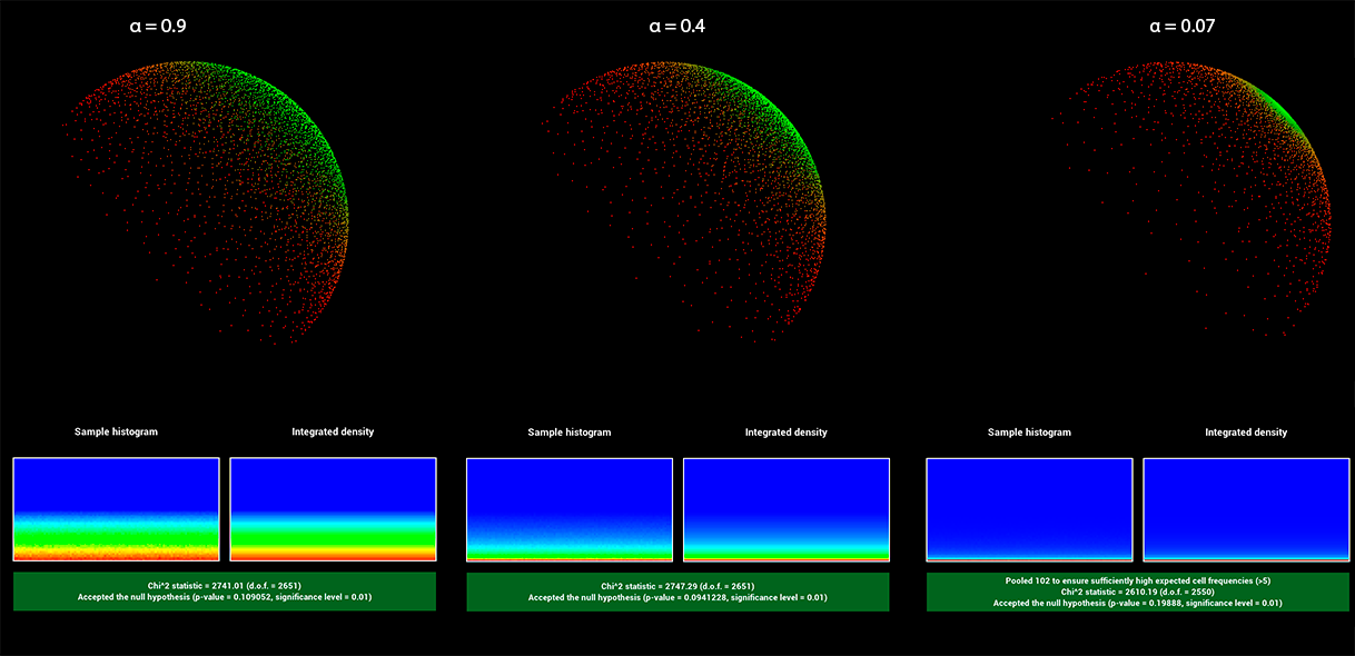
Homogeneous Medium
In order to render the particles in the water and the smoke of the cigar, I need to render volumetric participating media. Lets start with the homogeneous medium:
Sampling
The homogeneous medium supports importance sampling of the radiative transfer equation using the "sample" function. The method performs free path sampling to sample a distance t where it hits a particle and returns the throughput which is \(throughput = \sigma_s / \sigma_t \), since the transmittance and phase function and cancel out with the sampling probability.
Path Tracer
I implemented two versions of the path tracer. The first one is an extension of the path_mats.cpp and the second one an extension of path_mis.cpp. While looping over bounces the method keeps track of the medium the ray is currently in (can be null if no medium). As soon as we enter/leave a shape, which has an attached medium the current medium is changed.
Before the material or emitter sampling is happening, the path tracer checks if there is an intersection with a particle in the medium, which is done with the "sample" function in the medium class. If there is it updates the throughput and computes the next path using a phase function (isotropic or henyey-greenstein). If there is no particle intersection happening the method continues with a normal surface intersection.
For the multiple instance sampling path tracer, the emitter sampling has to be taken into account. In this case the shadowRay is traced and checked for intersections with shapes with surfaces. If the path goes through a medium the value is adjusted according to the transmittance of the medium.
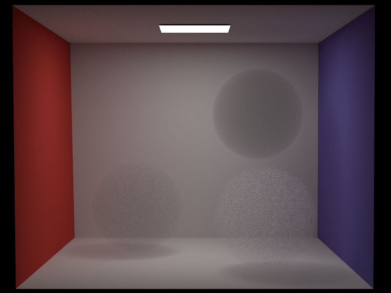
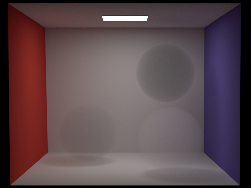
Isotropic Phase Function
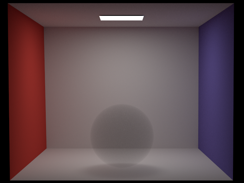
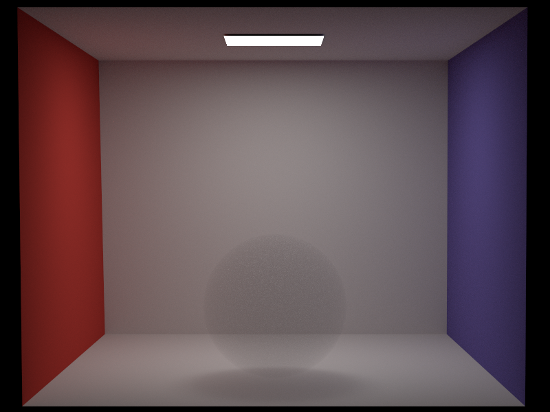
The isotropic phase function is a uniform distribution in all direction. It uses the Warp::squareToUniformSphere() function for sampling the direction and Warp::squareToUniformSpherePdf() to compute the probability. See below for a comparison of a medium rendered with the isotropic phase function in Nori and the one from Mitsuba. There are three spheres with different absorption and scattering values: bottom left - absorption = scattering = 0.5, bottom right - absorption = 0 and scattering = 1, top right - absorption = 1 and scattering = 0. The result is almost identical, the only difference is the noise in the medium, which might be caused due to a slighltly different multiple importance sampling strategy in Mitsuba.
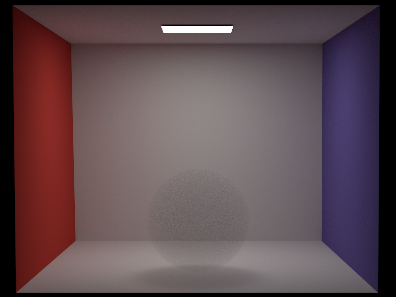
Henyey-Greenstein Phase Function
Using the henyey-greenstein phase function and the inversion method the following two equations can be derived to sample a direction: \[cos(\theta) = \frac{1}{2g} (1+g^2 - (\frac{1-g^2}{1-g+2g\xi_1})^2)\] \[\phi = 2\pi\xi_2\] See below for a comparison of Henyey-Greenstein with the Isotropic phase function: